Overview
In this project, we simulate natural lighting by tracing light rays in reverse (or "camera rays"). Standard ray-tracing with diffuse shading was implemented in Part 1 of this project.
Mirror and Glass Materials
We implemented the light-transfer functions for more complicated materials such as mirrors, glass, and "microfaceted" metals. Mirrors were simple, as we simply needed to reflect the incoming light ray across the surface normal. Glass was a bit more difficult, as we needed to perform a "coin flip" to decide whether to reflect the light or refract it through the glass. We also needed to check for cases of total internal reflection.
 Maximum ray depth 0
|
 Ray depth 1, some reflections showing.
|
 Ray depth 2, light rays refracting through glass sphere.
|
 Ray depth 3, light from source reflecting off ground beneath glass sphere.
|
 Ray depth 4, reflection off bottom of glass sphere and blue wall.
|
 Ray depth 100
|
Microfacet Materials
We implemented microfacet materials, which were a bit more complicated as we needed to "sample" a microsurface normal to reflect across, as well as calculate the Fresnel term. This last part in particular caused me problems, as I did not at first realize that we needed to calculate the term for each rgb channel independently.
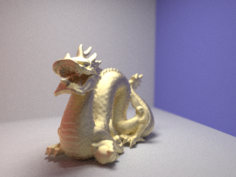
 Gold dragon, 0.005 alpha. Dull color, very small highlights.
|
 0.05 alpha. Brighter color, larger highlights, but increased noise in rest of image.
|
 0.25 alpha. Near perfect color and highlights, reduced noise.
|
 0.5 alpha. Still no noise, but colors far too bright.
|
 Copper bunny, cosine-weighted hemisphere sampling.
|
 Importance sampling. Convergence is much quicker, resulting in less noise.
|
 A titanium carbide dragon.
|
Environment Lighting
We implemented "environment lighting," where a 2d image is projected onto a sphere surrounding the scene we are rendering. To get the spectrum of light coming from a certain direction, we simply convert the direction of the light ray into a point on the image, and grab the color at that point. We also "bias" the incoming light rays towards the brighter parts of the image, so that more samples will fall on these bright regions. Calculating the probability distribution function for the environment light was not particularly complicated, but it was a good exercise in efficiency, as we had to find ways to avoid calculating the same values repeatedly.
 A field for environment lighting.
|
 A visual representation of the probability distribution.
|
 Uniform spherical sampling.
|
 Importance sampling. More noise, but the light samples are clearly biased towards one side of the bunny.
|
 Uniform spherical sampling.
|
 Importance sampling. Significantly more noise.
|
Depth of Field
We changed the simulation of our camera by including a "lens" whose diameter and focal length can be changed. In addition to sampling a direction to sample from, we also sample a point uniformly on the lens. The light ray that we actually sample starts at this point on the lens and points to where the original ray intersects the focal plane. This part was a bit challenging, as we had to do a lot of converting between "camera coordinates" and "world coordinates," as well as deciding which coordinate frame to perform our calculations in. In the end I chose to do the calculations in the world frame.
 Focal length 1
|
 Focal length 1.5
|
 Focal length 2
|
 Focal length 3
|
 Aperture size 0.02
|
 Aperture size 0.05
|
 Aperture size 0.1
|
 Aperture size 0.2
|